modist

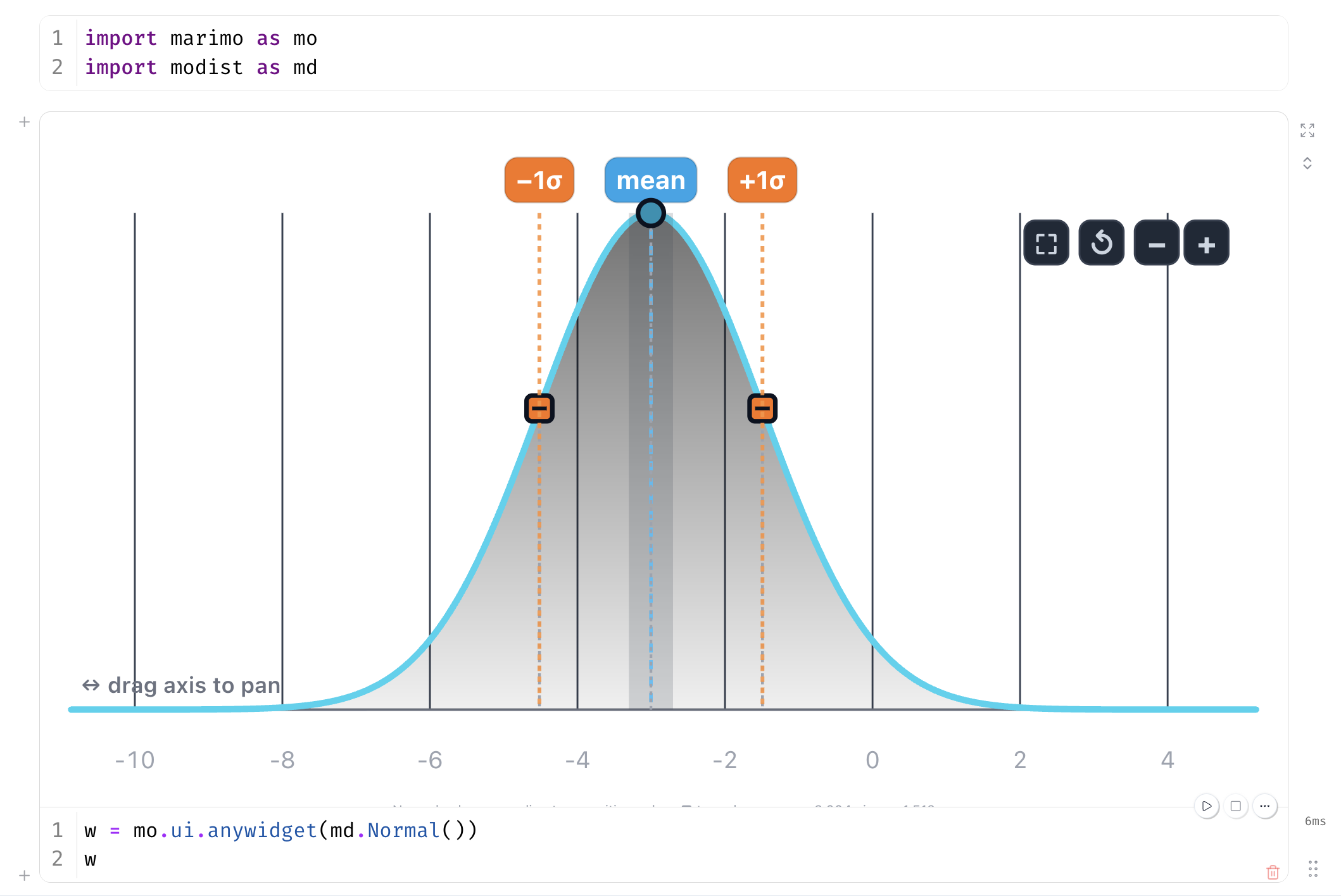
Interactive distribution widgets for marimo, in the style of koaning/wigglystuff. Drag the density curve to shape a distribution, then feed the params straight into a distribution constructor with a single splat.

Install

uv add modist            # or: uv pip install modist  (pip install modist)

The grouped-priors UI (md.ui) additionally requires marimo: uv add 'modist[marimo]' (or pip install modist[marimo]). The priors-from-model helpers (md.pymc) additionally require pymc: uv add 'modist[marimo,pymc]'.

Quickstart

import marimo as mo
import modist as md

w = mo.ui.anywidget(md.Normal())
w

params = w.value            # {'mu': ..., 'sigma': ...}

import pymc as pm
dist = pm.Normal.dist(**params)   # or pm.Beta / pm.Gamma / pm.StudentT

Priors UI

Allocate a whole set of priors at once with a tabbed panel — one draggable distribution per prior:

import modist as md

priors = {"intercept": md.Normal(), "slope": md.Normal(), "sigma": md.Gamma()}
ui = md.ui.create_tabs(priors)
ui

ui.value   # {'intercept': {'mu': ..., 'sigma': ...}, 'sigma': {'alpha': ..., 'beta': ...}, ...}

ui.value re-runs live as you drag, and each prior splats straight into its constructor: pm.Normal.dist(**ui.value["intercept"]). Use md.ui.create_tabs(priors, orientation="vertical") for a vertical tab bar, md.ui.create_tabs(priors, height=260) for shorter panels (the widgets size by aspect ratio, so a smaller height just narrows them), or md.ui.create_stack(priors) to show every prior at once.

ui.priors maps each name to a pymc_extras.Prior object (pip install pymc-extras). Your original distribution instances stay live as you drag, so symbolic flows built off them (w.create_variable(...), w.params, w.scipy) keep working.

Requires marimo (modist[marimo]). import modist itself stays marimo-free — md.ui is imported lazily on first access.

Priors from a PyMC model

Requires modist[marimo,pymc]. md.pymc is imported lazily, so plain import modist doesn't pull in pymc.

The same idea, lifted from a built model. md.pymc.create_priors(model) finds the model's root priors — distributions whose parameters don't depend on other distributions — replaces each with a draggable widget, compiles a sampler once, and bundles everything into a Priors panel you can drag, draw from, and hand straight to inference. The whole loop, from model to pm.sample, is one short session:

import numpy as np, pymc as pm, modist as md
x = np.random.default_rng(0).normal(size=(50, 3))
y = x @ [1.0, -0.5, 2.0] + np.random.default_rng(1).normal(size=50)

with pm.Model(coords={"covariate": ["retention", "content", "price"]}) as model:
    alpha = pm.Normal("alpha", mu=pm.Normal("alpha_mu", sigma=5), sigma=2)
    beta = pm.Normal("beta", dims="covariate")          # one widget per covariate
    sigma = pm.HalfNormal("sigma")                      # auto-mapped to a Gamma widget
    pm.Normal("obs", mu=alpha + x @ beta, sigma=sigma, observed=y)

ui = md.pymc.create_priors(model)   # tabs: alpha_mu, sigma, and a per-covariate beta group
ui                                    # drag the density curves to reshape the priors

Then use for prior predictive, etc:

ui.value                              # live params, ready to splat into pm.*.dist(**p)
ui.draw(1_000)                         # draws of every model RV, driven by the widgets
ui.draw(1_000, beta_price_mu=1.5)       # ... with a named per-parameter override
ui.sample_prior_predictive(1_000)       # -> xr.DataTree: prior / prior_predictive groups

Use the set_distributions method in order to define a new PyMC model.

new_model = ui.set_distributions()    # the widget families replace the priors
idata = pm.sample(model=new_model)    # ordinary pm.sample, ready for arviz

Families

Widget	Params	Domain	Drag affordances
Normal	mu, sigma	free	mean line → mu, ±1σ squares → sigma
Beta	alpha, beta	fixed [0, 1]	mean line → translate, q25/q75 squares → concentrate
Gamma	alpha, beta	edge pinned at 0	mean line → translate, q25/q75 squares → reshape
StudentT	mu, sigma, nu	free	mean line → mu, q75 square → sigma, tails dial → nu

StudentT's third parameter is a tails dial: drag it up for fatter tails (lower nu) or down for thinner tails (higher nu). Because nu has no natural on-curve landmark, its drag is a separate 1-D slider rather than a point you move on the density curve.

alpha/beta follow the PyMC / statistics convention (Gamma's beta is the rate, not scipy's scale). The lazy .scipy and .pymc adapters map to the right parametrization automatically:

n = md.Normal(mu=2.0, sigma=3.0)
n.scipy   # <scipy.stats.norm> via loc=/scale=
n.pymc    # pm.Normal.dist(mu=2.0, sigma=3.0)

g = md.Gamma(alpha=2.0, beta=3.0)
g.scipy   # scipy.stats.gamma(a=2.0, scale=1/3)  -- rate handled for you

w.value is a plain dict of the synced traits, so pm.X.dist(**w.value) works with no conversion.

Jupyter

The widgets are anywidget/ipywidgets under the hood, so they run in plain Jupyter too — no marimo required. Just display() the widget and read its .params (or .scipy) instead of wrapping it in mo.ui.anywidget(...):

import modist as md
from IPython.display import display

w = md.Normal(mu=0, sigma=1)
display(w)          # drag the curve to reshape it

w.params            # {'mu': ..., 'sigma': ...}

A full walkthrough notebook — all five families, live scipy stats, and a beta-prior combination example — lives at demos/jupyter_example.ipynb.

From a checkout:

uv sync --extra dev --extra scipy   # installs jupyter, ipykernel, jupytext
make jupyter                        # opens demos/jupyter_example.ipynb in JupyterLab

make jupyter registers the repo's .venv as a modist kernel, so the notebook uses exactly the installed packages. Requires a local JupyterLab (installed alongside jupyter via the dev extras).

How it works

Each family is its own anywidget class with a small set of synced parameter traits (no x_min/x_max/n_points). The view — SVG scaffold, pan/zoom, draggable hit lines, and per-family math — lives in a self-contained ESM module.

Source JS lives in js/ (js/base.js shared scaffold + one family file, all importing a vendored copy of jStat for pdf/cdf/quantile math). Anywidget delivers _esm as a Blob URL, which cannot resolve relative imports, so esbuild bundles each family (jStat inlined) into the committed src/modist/static/*.js files — the same pattern wigglystuff uses for its JS-heavy widgets.

Rebuilding the JS

make js          # esbuild js/*.js -> src/modist/static/*.js
make js-watch    # rebuild on every edit (for anywidget hot-reload dev)

Requires a local esbuild (npm install --no-save esbuild).

Development

make venv        # creates .venv with dev deps + esbuild
make test        # pytest
npm run test:js  # Playwright JS integration probes (headless Chromium)

Acknowledgements

• jStat — JavaScript statistics library (MIT), vendored and bundled for the pdf/cdf/quantile math.
• wigglystuff — the interaction and architecture model (one class per family, prebuilt ESM per class).