torch-harmonics

Overview

torch-harmonics implements differentiable signal processing on the sphere. This includes differentiable implementations of the spherical harmonic transforms, vector spherical harmonic transforms and discrete-continuous convolutions on the sphere. The package was originally implemented to enable Spherical Fourier Neural Operators (SFNO) [1]. A description of the library as a whole is given in [7].

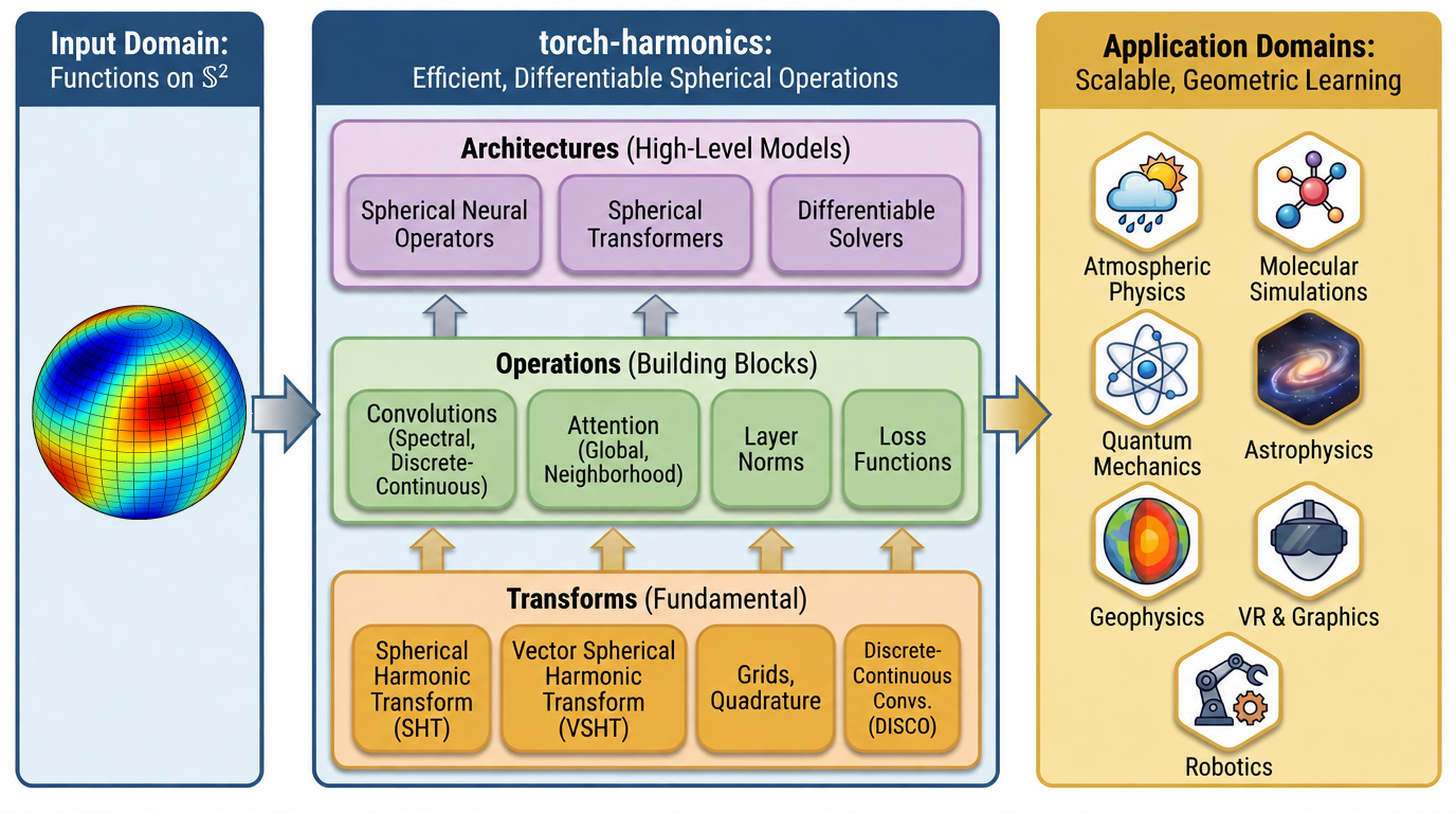
The SHT algorithm uses quadrature rules to compute the projection onto the associated Legendre polynomials and FFTs for the projection onto the harmonic basis. This algorithm tends to outperform others with better asymptotic scaling for most practical purposes [2].

torch-harmonics uses PyTorch primitives to implement these operations, making it fully differentiable. Moreover, the quadrature can be distributed onto multiple ranks making it spatially distributed.

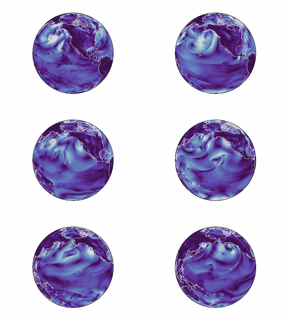
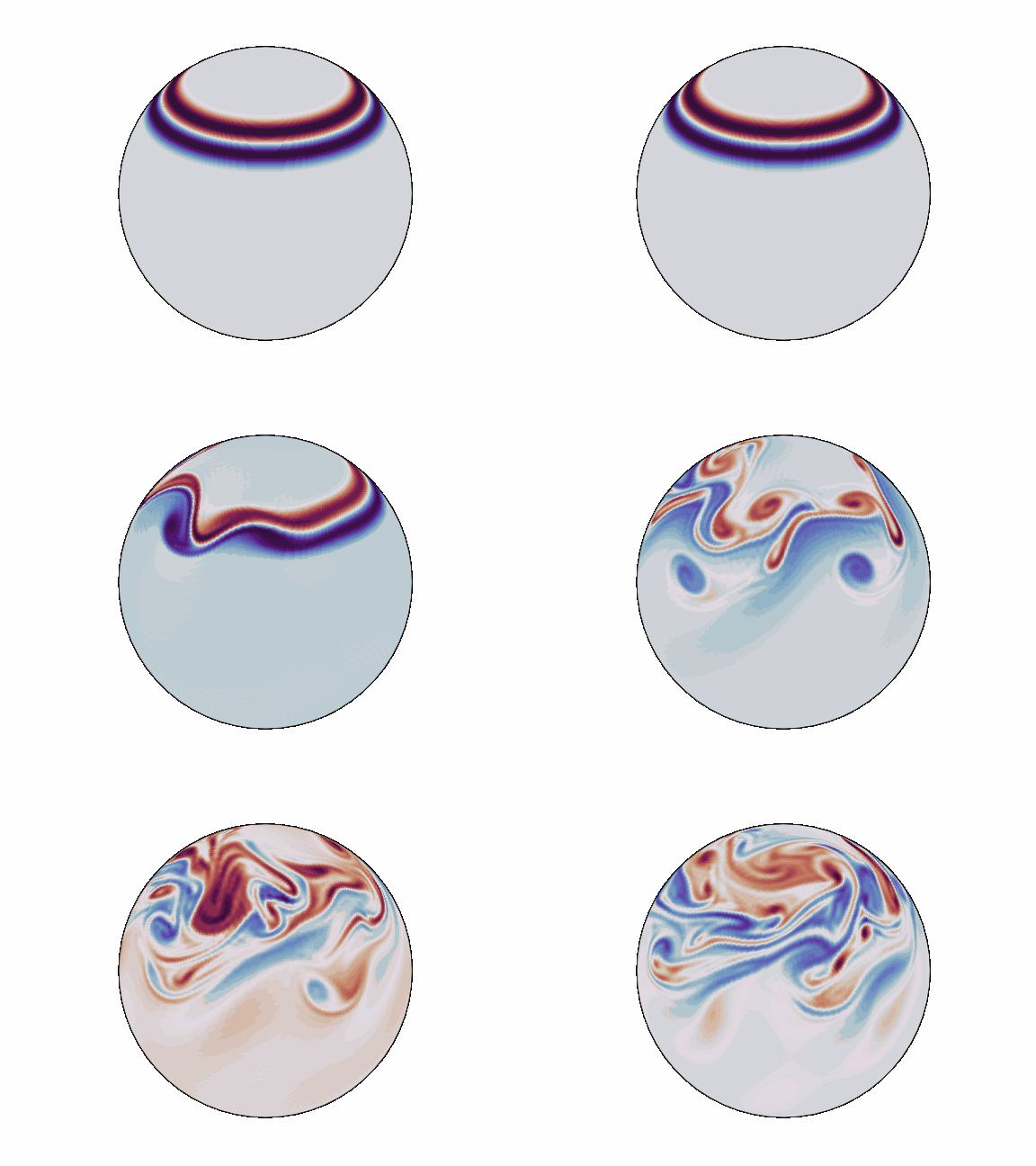
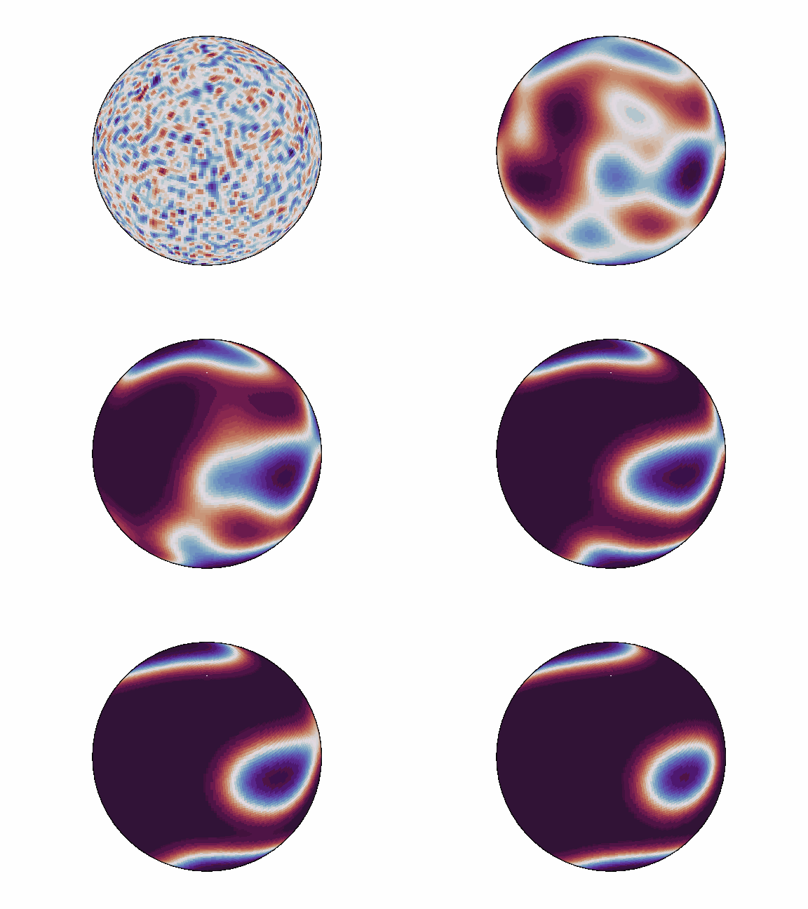
torch-harmonics has been used to implement a variety of differentiable PDE solvers which generated the animations below. Moreover, it has enabled the development of Spherical Fourier Neural Operators [1].

Installation

Prebuilt wheels

Prebuilt Linux wheels with compiled CUDA extensions are available on pypi.nvidia.com. Pick the package matching your CUDA toolkit version:

CUDA	Package	Supported PyTorch	Install command
12.6	`torch-harmonics-cu126`	2.9.1	`pip install torch-harmonics-cu126 --extra-index-url https://pypi.nvidia.com`
12.8	`torch-harmonics-cu128`	2.9.1	`pip install torch-harmonics-cu128 --extra-index-url https://pypi.nvidia.com`
12.9	`torch-harmonics-cu129`	2.9.1	`pip install torch-harmonics-cu129 --extra-index-url https://pypi.nvidia.com`
13.0	`torch-harmonics-cu130`	2.9.1	`pip install torch-harmonics-cu130 --extra-index-url https://pypi.nvidia.com`
13.2	`torch-harmonics-cu132`	2.12.0	`pip install torch-harmonics-cu132 --extra-index-url https://pypi.nvidia.com`

If you don't need a specific CUDA version, use the rolling alias for the latest CUDA build:

pip install torch-harmonics-cuda-latest --extra-index-url https://pypi.nvidia.com

For a CPU-only build, install the torch-harmonics package from PyPI.

Tip: Run nvidia-smi to check your driver's CUDA version.

Older PyTorch or CUDA (PyTorch before 2.9, CUDA before 12.6) have no prebuilt wheels. Use the Docker container, which brings a matching PyTorch and CUDA, or build torch-harmonics from source against your installed PyTorch, adding --no-deps so that pip does not replace it with a newer one (pip install --no-build-isolation --no-deps .). These combinations are not tested.

PyPI

The vanilla torch-harmonics package on PyPI ships a CPU-only prebuilt wheel. This version is built for the newest PyTorch release. For GPU support, use the NVIDIA PyPI packages above.

pip install torch-harmonics

Building from source

If your OS, PyTorch or CUDA toolkit version is not covered by the available wheels, we recomment building torch-harmonics from the GitHub repository. Use --no-build-isolation so that custom CPU and CUDA kernels compile against your existing torch installation:

git clone git@github.com:NVIDIA/torch-harmonics.git
cd torch-harmonics
pip install --no-build-isolation -e .

If CUDA devices are not detected automatically (e.g. inside a container), set the TORCH_HARMONICS_BUILD_CUDA_EXTENSION flag. Set TORCH_CUDA_ARCH_LIST to only the architectures you need to reduce compilation time:

export TORCH_HARMONICS_BUILD_CUDA_EXTENSION=1
export TORCH_CUDA_ARCH_LIST="8.0 8.6 9.0a 10.0a+PTX"
pip install --no-build-isolation -e .

Tip: Use the a suffix (e.g. 9.0a, 10.0a) instead of plain 9.0 or 10.0 to enable architecture-specific tensor core instructions (e.g. wgmma on Hopper). Some layers such as DISCO benefit significantly from this. The trade-off is that the resulting binary is only compatible with the exact GPU generation it was compiled for.

⚠️ Custom CUDA extensions require architectures >= 7.0.

Alternatively, build a Docker container:

git clone git@github.com:NVIDIA/torch-harmonics.git
cd torch-harmonics
docker build . -t torch_harmonics
docker run --gpus all -it --rm --ipc=host --ulimit memlock=-1 --ulimit stack=67108864 torch_harmonics

More about torch-harmonics

Spherical harmonics

The spherical harmonics are special functions defined on the two-dimensional sphere $S^2$ (embedded in three dimensions). They form an orthonormal basis of the space of square-integrable functions defined on the sphere $L^2(S^2)$ and are comparable to the harmonic functions defined on a circle/torus. The spherical harmonics are defined as

$$ Y_l^m(\theta, \lambda) = \sqrt{\frac{(2l + 1)}{4 \pi} \frac{(l - m)!}{(l + m)!}} P_l^m(\cos \theta) \exp(im\lambda), $$

where $\theta$ and $\lambda$ are colatitude and longitude respectively, and $P_l^m$ the normalized, associated Legendre polynomials.

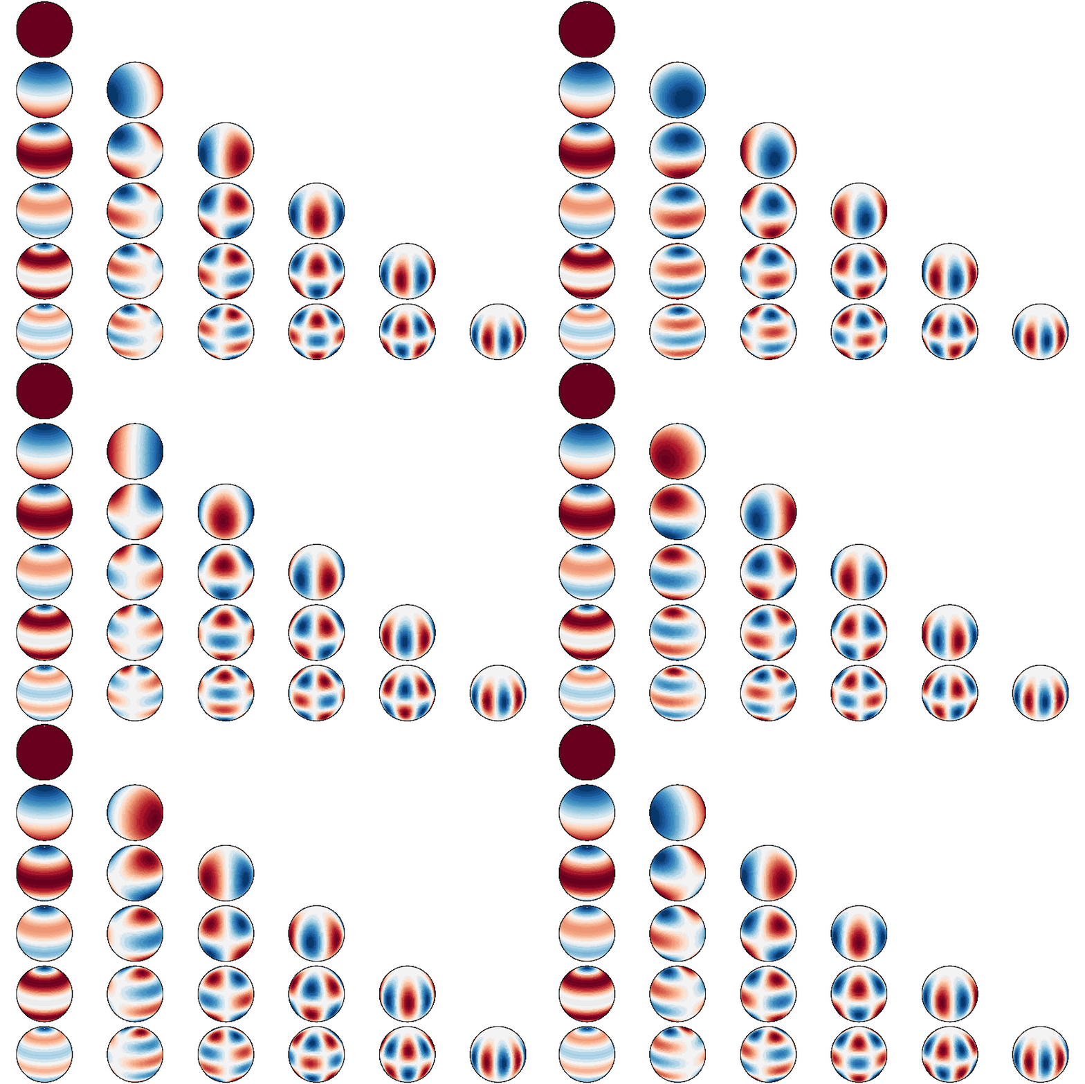
Spherical harmonics up to degree 5

Spherical harmonic transform

The spherical harmonic transform (SHT)

$$ f_l^m = \int_{S^2} \overline{Y_{l}^{m}}(\theta, \lambda) f(\theta, \lambda) \mathrm{d} \mu(\theta, \lambda) $$

realizes the projection of a signal $f(\theta, \lambda)$ on $S^2$ onto the spherical harmonics basis. The SHT generalizes the Fourier transform on the sphere. Conversely, a truncated series expansion of a function $f$ can be written in terms of spherical harmonics as

$$ f (\theta, \lambda) = \sum_{m=-M}^{M} \exp(im\lambda) \sum_{l=|m|}^{M} \hat f_l^m P_l^m (\cos \theta), $$

where $\hat{f}_l^m$, are the expansion coefficients associated to the mode $m$, $n$.

The implementation of the SHT follows the algorithm as presented in [2]. A direct spherical harmonic transform can be accomplished by a Fourier transform

$$ \hat f^m(\theta) = \frac{1}{2 \pi} \int_{0}^{2\pi} f(\theta, \lambda) \exp(-im\lambda) \mathrm{d} \lambda $$

in longitude and a Legendre transform

$$ \hat f_l^m = \frac{1}{2} \int^{\pi}_0 \hat f^{m} (\theta) P_l^m (\cos \theta) \sin \theta \mathrm{d} \theta $$

in latitude.

Discrete Legendre transform

The second integral, which computed the projection onto the Legendre polynomials is realized with quadrature. On the Gaussian grid, we use Gaussian quadrature in the $\cos \theta$ domain. The integral

$$ \hat f_l^m = \frac{1}{2} \int_{-1}^1 \hat{f}^m(\arccos x) P_l^m (x) \mathrm{d} x $$

is obtained with the substitution $x = \cos \theta$ and then approximated by the sum

$$ \hat f_l^m = \sum_{j=1}^{N_\theta} \hat{f}^m(\arccos x_j) P_l^m(x_j) w_j. $$

Here, $x_j \in [-1,1]$ are the quadrature nodes with the respective quadrature weights $w_j$.

Discrete-continuous convolutions on the sphere

torch-harmonics now provides local discrete-continuous (DISCO) convolutions as outlined in [5] on the sphere. These are use in local neural operators [2] to generalize convolutions to structured and unstructured meshes on the sphere.

Spherical (neighborhood) attention

torch-harmonics introduces spherical attention mechanisms which correctly generalize the attention mechanism to the sphere. The use of quadrature rules makes the resulting operations approximately equivariant and equivariant in the continuous limit. Moreover, neighborhood attention is correctly generalized onto the sphere by using the geodesic distance to determine the size of the neighborhood.

Getting started

The main functionality of torch_harmonics is provided in the form of torch.nn.Modules for composability. A minimum example is given by:

import torch
import torch_harmonics as th

device = torch.device('cuda' if torch.cuda.is_available() else 'cpu')

nlat = 512
nlon = 2*nlat
batch_size = 32
signal = torch.randn(batch_size, nlat, nlon, device=device)

# transform data on an equiangular grid
grid = th.EquiangularGrid(nlat=nlat, nlon=nlon)
sht = th.RealSHT(grid).to(device)

coeffs = sht(signal)

Grids

Every layer takes a grid descriptor rather than a resolution and a grid name. The descriptor holds both, along with everything that follows from where the nodes sit: the quadrature weights, the node spacing localized operators take their default cutoff from, and the degree an SHT can be truncated to without losing orthogonality. Each grid type has its own class, e.g. th.EquiangularGrid(nlat=..., nlon=...) or th.HealpixGrid(nside=...). Alternatively, th.as_grid builds a grid from its name, e.g. th.as_grid("equiangular", nlat=..., nlon=...), which is convenient when the grid type comes from a configuration file.

The supported grids differ in where they place their nodes, which the figure below shows at coarse resolution, both on the sphere and in longitude-latitude coordinates:

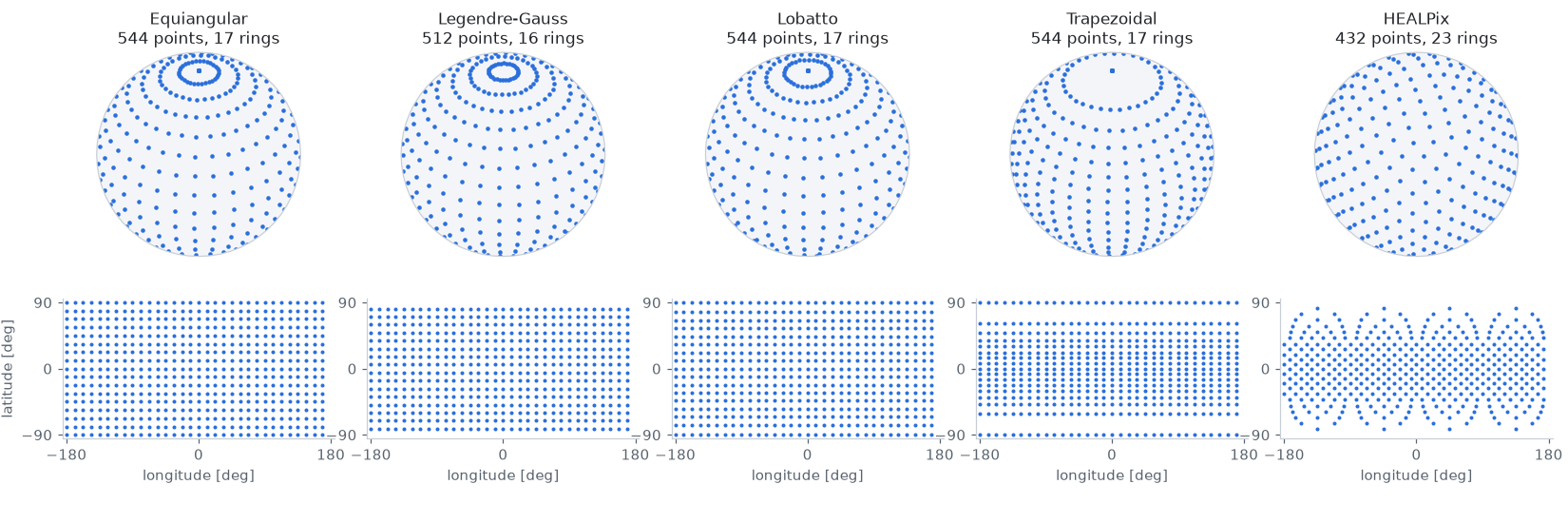
Equiangular: rings equally spaced in latitude, including both poles, with Clenshaw-Curtis quadrature. This is the familiar latitude-longitude grid used for most reanalysis and climate data.
Legendre-Gauss: rings at the roots of the Legendre polynomial in $\cos\theta$, excluding the poles. Gaussian quadrature is exact up to the highest polynomial degree for a given number of rings, so this grid supports the highest SHT bandlimit per ring.
Lobatto: Gauss-Lobatto nodes, i.e. Legendre-Gauss-like rings that include both poles.
Trapezoidal: rings equally spaced in $\cos\theta$ with the trapezoidal rule, which places them densely near the equator and sparsely near the poles. Its quadrature converges only algebraically, so it is suited for quadrature and localized operators but not for an SHT at a high bandlimit.
HEALPix [8]: 12 * nside**2 pixels of equal area on 4 * nside - 1 rings of constant latitude. The rings have different lengths, so a field is stored as a flat tensor of shape (..., npix) in RING order. HEALPix supports attention, DISCO convolutions and quadrature but not the SHT yet.

grid type	class	field shape	accepted by
`"equiangular"`	`th.EquiangularGrid(nlat=..., nlon=...)`	`(nlat, nlon)`	every layer
`"legendre-gauss"`	`th.LegendreGaussGrid(nlat=..., nlon=...)`	`(nlat, nlon)`	every layer
`"lobatto"`	`th.LobattoGrid(nlat=..., nlon=...)`	`(nlat, nlon)`	every layer
`"trapezoidal"`	`th.TrapezoidalGrid(nlat=..., nlon=...)`	`(nlat, nlon)`	every layer
`"healpix"`	`th.HealpixGrid(nside=...)`	`(npix,)`	`AttentionS2`, `NeighborhoodAttentionS2`, `DiscreteContinuousConvS2`, `DiscreteContinuousConvTransposeS2`, `QuadratureS2`

Layers that map between two grids take grid_in and grid_out, which need not be of the same type -- attention can decode from HEALPix onto a latitude-longitude grid, for instance:

hp = th.HealpixGrid(nside=16)                          # 3072 equal-area pixels
ll = th.EquiangularGrid(nlat=33, nlon=64)

attn = th.NeighborhoodAttentionS2(grid_in=hp, grid_out=hp, in_channels=32, num_heads=4)
decode = th.AttentionS2(grid_in=hp, grid_out=ll, in_channels=32, num_heads=4)

x = torch.randn(2, 32, hp.npoints)                     # a HEALPix field is flat: (..., npix)
h = attn(x)                                            # self-attention: (2, 32, 3072)

q = torch.randn(2, 32, 33, 64)                         # queries live on the output grid,
y = decode(q, key=h, value=h)                          # keys and values on the input grid

Volumetric fields on balls, shells or the space outside a sphere use a radial grid together with any of the grids above. th.SphericalProductGrid(angular, radial) samples the same angular grid at every radius, and a field on it is laid out (..., nr, *angular.shape). Every layer accepts a product grid and acts on each shell alike, treating the radius as a batch axis. th.QuadratureVolume integrates over the volume:

shells = th.LegendreGaussRadialGrid(nr=8, r_inner=1.0, r_outer=2.0)
grid = th.SphericalProductGrid(th.EquiangularGrid(nlat=33, nlon=64), shells)   # grid.shape == (8, 33, 64)

conv = th.DiscreteContinuousConvS2(grid_in=grid, grid_out=grid, in_channels=4, out_channels=8, kernel_shape=3)
x = torch.randn(2, 4, *grid.shape)                     # (batch, channels, nr, nlat, nlon)
y = conv(x)                                            # every shell convolved alike: (2, 8, 8, 33, 64)

volume = th.QuadratureVolume(grid)(torch.ones(grid.shape))   # 4/3 pi (2^3 - 1^3)

The distributed layers take the global grid and derive each rank's shard from it. Passing a resolution where a descriptor belongs raises a TypeError naming the replacement, and a layer that does not support a grid yet refuses it at construction. See Grids for the full descriptor API, and the grid descriptors notebook for a walkthrough.

Distributed and further reading

To enable scalable model-parallelism, torch-harmonics implements a distributed variant of the SHT located in torch_harmonics.distributed.

Detailed usage of torch-harmonics, alongside helpful analysis provided in a series of notebooks:

Benchmarks

The benchmarks/ directory contains a performance benchmark suite covering SHT, DISCO convolution, and spherical attention across resolutions, dtypes, and channel counts.

# run full suite on current GPU
python benchmarks/run.py

# filter by name or tag
python benchmarks/run.py --name disco
python benchmarks/run.py --tags attention neighborhood

# save a baseline, then compare after a change
python benchmarks/run.py --save-csv before.csv
python benchmarks/run.py --reference-csv before.csv

See CONTRIBUTING.md for the full workflow expected in performance-related PRs.

Examples and reproducibility

The examples folder contains training scripts for three distinct tasks:

Results from the papers can generally be reproduced by running python train.py. In the case of some older results the number of epochs and learning-rate may need to be adjusted by passing the corresponding command line argument.

Remarks on automatic mixed precision (AMP) support

Note that torch-harmonics uses Fourier transforms from torch.fft which in turn uses kernels from the optimized cuFFT library. This library supports fourier transforms of float32 and float64 (i.e. single and double precision) tensors for all input sizes. For float16 (i.e. half precision) and bfloat16 inputs however, the dimensions which are transformed are restricted to powers of two. Since data is converted to one of these reduced precision floating point formats when torch.autocast is used, torch-harmonics will issue an error when the input shapes are not powers of two. For these cases, we recommend disabling autocast for the harmonics transform specifically:

import torch
import torch_harmonics as th

sht = th.RealSHT(th.EquiangularGrid(nlat=512, nlon=1024)).cuda()

with torch.autocast(device_type="cuda", enabled = True):
   # do some AMP converted math here
   x = some_math(x)
   # convert tensor to float32
   x = x.to(torch.float32)
   # now disable autocast specifically for the transform,
   # making sure that the tensors are not converted
   # back to reduced precision internally
   with torch.autocast(device_type="cuda", enabled = False):
      xt = sht(x)

   # continue operating on the transformed tensor
   xt = some_more_math(xt)

Depending on the problem, it might be beneficial to upcast data to float64 instead of float32 precision for numerical stability.

Contributors

Boris Bonev (bbonev@nvidia.com), Thorsten Kurth (tkurth@nvidia.com), Max Rietmann, Mauro Bisson, Andrea Paris, Alberto Carpentieri, Massimiliano Fatica, Nikola Kovachki, Jean Kossaifi, Christian Hundt

Cite us

If you use torch-harmonics in your work, please cite the paper describing the library [7]:

@misc{kurth2026library,
      title={A library for differentiable signal processing and machine learning on the sphere},
      author={Thorsten Kurth and Max Rietmann and Mauro Bisson and Andrea Paris and Alberto Carpentieri and Jean Kossaifi and Anima Anandkumar and Christian Hundt and Boris Bonev},
      year={2026},
      eprint={2609.39737},
      archivePrefix={arXiv},
      primaryClass={cs.LG},
      url={https://arxiv.org/abs/2609.39737}
}

If you use the spherical neural operators or spherical attention, please also cite the papers introducing them: Spherical Fourier Neural Operators [1], localized neural operators with discrete-continuous convolutions [2], and attention on the sphere [6]:

@misc{bonev2023spherical,
      title={Spherical Fourier Neural Operators: Learning Stable Dynamics on the Sphere},
      author={Boris Bonev and Thorsten Kurth and Christian Hundt and Jaideep Pathak and Maximilian Baust and Karthik Kashinath and Anima Anandkumar},
      year={2023},
      eprint={2306.03838},
      archivePrefix={arXiv},
      primaryClass={cs.LG}
}

@misc{liuschiaffini2024neural,
      title={Neural Operators with Localized Integral and Differential Kernels},
      author={Miguel Liu-Schiaffini and Julius Berner and Boris Bonev and Thorsten Kurth and Kamyar Azizzadenesheli and Anima Anandkumar},
      year={2024},
      eprint={2402.16845},
      archivePrefix={arXiv},
      primaryClass={cs.LG}
}

@misc{bonev2025attention,
      title={Attention on the Sphere},
      author={Boris Bonev and Max Rietmann and Andrea Paris and Alberto Carpentieri and Thorsten Kurth},
      year={2025},
      eprint={2505.11157},
      archivePrefix={arXiv},
      primaryClass={cs.LG}
}

References

[1] Bonev B., Kurth T., Hundt C., Pathak, J., Baust M., Kashinath K., Anandkumar A.; Spherical Fourier Neural Operators: Learning Stable Dynamics on the Sphere; International Conference on Machine Learning, 2023. arxiv link

[2] Liu-Schiaffini M., Berner J., Bonev B., Kurth T., Azizzadenesheli K., Anandkumar A.; Neural Operators with Localized Integral and Differential Kernels; International Conference on Machine Learning, 2024. arxiv link

[3] Schaeffer N.; Efficient spherical harmonic transforms aimed at pseudospectral numerical simulations; G3: Geochemistry, Geophysics, Geosystems, 2013.

[4] Wang B., Wang L., Xie Z.; Accurate calculation of spherical and vector spherical harmonic expansions via spectral element grids; Adv Comput Math, 2018.

[5] Ocampo, Price, McEwen, Scalable and equivariant spherical CNNs by discrete-continuous (DISCO) convolutions, ICLR (2023), arXiv:2209.13603

[6] Bonev B., Rietmann M., Paris A., Carpentieri A., Kurth T.; Attention on the Sphere; arxiv link

[7] Kurth T., Rietmann M., Bisson M., Paris A., Carpentieri A., Kossaifi J., Anandkumar A., Hundt C., Bonev B.; A library for differentiable signal processing and machine learning on the sphere; arXiv preprint, 2026. arxiv link

[8] Gorski K. M., Hivon E., Banday A. J., Wandelt B. D., Hansen F. K., Reinecke M., Bartelmann M.; HEALPix: A Framework for High-Resolution Discretization and Fast Analysis of Data Distributed on the Sphere; The Astrophysical Journal, 622:759-771, 2005.

Name		Name	Last commit message	Last commit date
.github		.github
.skills		.skills
benchmarks		benchmarks
docs		docs
examples		examples
images		images
notebooks		notebooks
scripts		scripts
tests		tests
torch_harmonics		torch_harmonics
.clang-format		.clang-format
.clang-format-ignore		.clang-format-ignore
.coveragerc		.coveragerc
.gitattributes		.gitattributes
.gitignore		.gitignore
.pre-commit-config.yaml		.pre-commit-config.yaml
.readthedocs.yaml		.readthedocs.yaml
AUTHORS		AUTHORS
CONTRIBUTING.md		CONTRIBUTING.md
Changelog.md		Changelog.md
Dockerfile		Dockerfile
Dockerfile.examples		Dockerfile.examples
LICENSE.txt		LICENSE.txt
README.md		README.md
SECURITY.md		SECURITY.md
SKILL.md		SKILL.md
pyproject.toml		pyproject.toml
setup.py		setup.py

Navigation Menu

Repository navigation

About

Repository files navigation

torch-harmonics

Overview

Installation

Prebuilt wheels

PyPI

Building from source

More about torch-harmonics

Spherical harmonics

Spherical harmonic transform

Discrete Legendre transform

Discrete-continuous convolutions on the sphere

Spherical (neighborhood) attention

Getting started

Grids

Distributed and further reading

Benchmarks

Examples and reproducibility

Remarks on automatic mixed precision (AMP) support

Contributors

Cite us

References

About

Releases

Packages

Used by

Contributors

Languages

Latest commit

History

Folders and files

Repository files navigation

torch-harmonics

Overview

Installation

Prebuilt wheels

PyPI

Building from source

More about torch-harmonics

Spherical harmonics

Spherical harmonic transform

Discrete Legendre transform

Discrete-continuous convolutions on the sphere

Spherical (neighborhood) attention

Getting started

Grids

Distributed and further reading

Benchmarks

Examples and reproducibility

Remarks on automatic mixed precision (AMP) support

Contributors

Cite us

References

About

Topics

Resources

Contributing

Security policy

Stars

Watchers

Forks

Releases

Packages

Used by

Contributors

Languages